Feynman-Kac plugin description

This plugin solves Exercise 2.2 of the "Introduction to Parallel Computing" book described at page 82 [1].

We solve a partial differential equation inside an elliptical region by Monte Carlo simulations of the Feynman-Kac formula. The following partial differential equation is defined in a three-dimensional ellipsoid E:

$$\frac{1}{2}\triangle u(x,y,z)-v(x,y,z)u(x,y,z)=0,$$

where the ellipsoidal domain is

$$D= \Bigg\{(x,y,z) \in \mathbf{R}^3; \frac{x^2}{a^2}+\frac{y^2}{b^2}+\frac{z^2}{c^2} < 1 \Bigg\}.$$

The potential is

$$v(x,y,z) = 2(\frac{x^2}{a^4}+\frac{y^2}{b^4}+\frac{z^2}{c^4}+\frac{1}{a^2}+\frac{1}{b^2}+\frac{1}{c^2}).$$

Our Dirichlet boundary condition is $u=g(\mathbf{x})=1$ when $\mathbf{x} \in \partial{D}.$

The goal is to solve this boundary value problem at $\mathbf{x}=(x,y,z)$ by a Monte Carlo simulation. At the heart of the simulation lies the Feynman-Kac formula, which in our case ($g=1$) is

$$u(x,y,z) = \mathbf{E} \; g(\mathbf{X}(\tau)) \; exp\Bigg(-\int_{0}^{\tau}v(\mathbf{X}(s))ds \Bigg)$$

$$u(x,y,z) = \mathbf{E} \; exp\Bigg(-\int_{0}^{\tau}v(\mathbf{X}(s))ds \Bigg)$$

$$u(x,y,z) = \mathbf{E} \; Y(\tau).$$

which describes the solution $u$ in terms of an expectation value of a stochastic process $Y$ whose initial value $Y(0)=1$. Here $\mathbf{X}(s)$ is a Brownian motion starting from $\mathbf{X}(0)=\mathbf{x}$ and $\tau$ is its exit time from $D$.

It is important to point out that the $\mathbf{E}$ operator in simulation means $\mathbf{E} f = \frac{1}{N} \sum_{i=1}^{N} f_{i}$ for samples of size $N$.

The plugin pde3d.dll can be called in two different ways:

0,[a],[b],[c],feynmankac3d
1,[a],[b],[c],[initialx],[initialy],[initialz],feynmankac3d

The first call passes the ellipses axes as parameter. The function
feynmankac3d stored in pde3d.dll generates first randomly a point $\mathbf{x}$ inside the ellipse. In the second call, we can specify the initial

$$\mathbf{x}=([initialx],[initialy],[initialz]).$$

0 or 1 inform the plugin on how many parameters are loaded on the stack.

From this initial interior point $\mathbf{X}(0)=\mathbf{x} \in D$ we integrate the following system of stochastic differential equations ( $\mathbf{W}$ is a Brownian motion). We use $N$ realizations of $\mathbf{X}(t)$ to integrate.

$$d\mathbf{X} = d\mathbf{W}$$

$$dY = -v(\mathbf{X}(t))Ydt$$

For each realization, we integrate this set of equations until $\mathbf{X}(t)$ exits at time $t=\tau$ using the trapezoidal rule [1]. Finally, we compute $u(\mathbf{x})=\mathbf{E}Y(\mathbf{X}(\tau))$ to get the solution.

To plot the error, we compare it to the exact analytical solution of the partial differential equation, computed by two differentiations:

$$u(x,y,z)=exp(\frac{x^2}{a^2}+\frac{y^2}{b^2}+\frac{z^2}{c^2}-1).$$

The error in the plugin's graphical output is plotted as an oscillating green line around the y axis. After oscillating for a while, the error tends to converge to the y axis. Only one out of many random walks ( $\mathbf{X}(t)$) is plotted with red or white colors.

Roughly speaking, we free a horde of random walkers from an initial point. These walkers diffuse while $Y$ is integrated with rate $-v(\mathbf{X})$ on the potential $v$ until they reach the boundary of the ellipse. All walks are averaged in a similar way as it is done with the pi plugin to get the function value at the chosen initial point. The diffusion process of the walkers, distributed as a trivariate normal density, weights points near the initial point more than points far away.

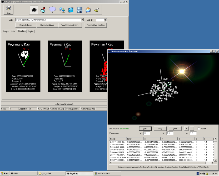
Figure 13: GPU computing the Feynman-Kac problem and corresponding frontend.